Simulation-based inference (SBI) acceleration

In this tutorial you will learn:

How to specify a mock data generator in addition to the likelihood
How to train a simulation-based inference model to predict a posterior distribution (neural posterior estimation)
How to verify that the simulation-based inference trained well
How to use SBI-NPE to accelerate the UltraNest nested sampling run

In this example, we fit a Voigt line in a spectrum.

[1]:

import numpy as np
import matplotlib.pyplot as plt
import corner
import ultranest
import ultranest.simbase.minisbi

rng = np.random.default_rng(123)

Defining the model

Gaussian measurement noise

First, we need our physical model function of the intrinsic spectrum, and also predict the noise level. We assume a Voigt line shape and constant noise.

[2]:

noise_std = 0.1

[3]:

N_DATA = 1000
x = np.geomspace(0.55, 0.75, N_DATA)

[4]:

parameter_names = ["amplitude", "center_x", "width", "background", "slope"]
N_PARAMS = len(parameter_names)

Define the model spectrum function, given model parameters

[5]:

from scipy.special import voigt_profile

[6]:

sigma_instrumental = 0.001 # nominal resolution of the spectrograph

[7]:

def generate_mean_and_noise(theta, idx=0, seed=0):
    amplitude, center_x, width, background, slope = theta
    signal = amplitude * voigt_profile(x - center_x, sigma_instrumental, width) + background + (x / center_x) ** slope

    return {
        'mean':      signal,
        'noise_std': signal * 0 + noise_std,  # same noise for each data point
    }

The received idx and seed are not used here. They are integers, in case randomness in the physics model is needed.

Our true parameters for this example:

[8]:

theta_true = [0.0042, 0.656279, 0.001, 0.2, -1.]

[9]:

plt.errorbar(
    x=x,
    y=generate_mean_and_noise(theta_true)['mean'],
    capsize=0,
)
plt.fill_between(
    x,
    generate_mean_and_noise(theta_true)['mean'] - generate_mean_and_noise(theta_true)['noise_std'],
    generate_mean_and_noise(theta_true)['mean'] + generate_mean_and_noise(theta_true)['noise_std'],
    alpha=0.1,
)
plt.yscale('log');

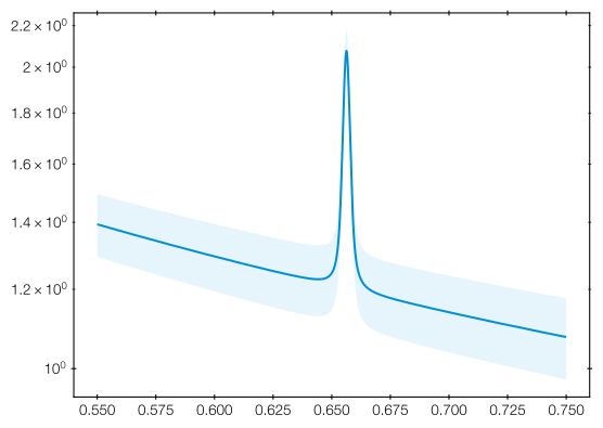
_images/example-simulation-based-inference_15_0.svg

A beautiful spectrum of a line, on top of a slightly sloped continuum.

Prior distribution

Define our prior distribution as usual, based on unit cube transforms.

[10]:

def prior_transform(u):
    result = u.copy()
    # amplitude (index 0): log-uniform [1e-2, 1e2]
    result[0] = 10**(-4 + u[0] * 4)
    # center_x (index 1): uniform [0.65, 0.66]
    result[1] = 0.65 + u[1] * 0.01
    # width (index 2): uniform [1e-4, 0.01]
    result[2] = 10**(-4 + 2 * u[2])
    # background level (index 3): uniform [-1, 1]
    result[3] = -1 + 2 * u[3]
    # slope (index 4): uniform [-2, +2]
    result[4] = -2 + 4 * u[4]
    return result

Generate noisy data

The observed data we will fit

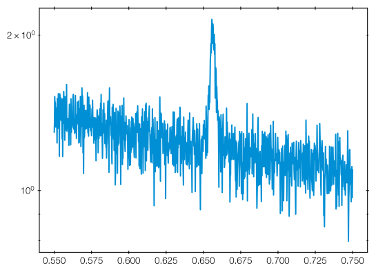
Going from the model above to data is trivial, with a Gaussian random number generator:

[11]:

def inject_noise(mean_props, rng):
    return rng.normal(mean_props['mean'], mean_props['noise_std'])

[12]:

obs_spectrum = inject_noise(generate_mean_and_noise(theta_true), rng)

plt.plot(x, obs_spectrum)
plt.yscale('log')

_images/example-simulation-based-inference_24_0.svg

Generate mock data - Prior predictive checks

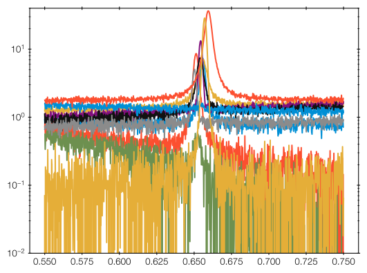
Here are some example data sets when we sampled from the prior. These show the diversity of data we consider reasonable a priori:

[13]:

for i in range(10):
    u = rng.uniform(size=N_PARAMS)
    params = prior_transform(u)
    plt.plot(x, inject_noise(generate_mean_and_noise(params), rng))
    plt.yscale('log')
    plt.ylim(1e-2, 40)

_images/example-simulation-based-inference_27_0.svg

Data likelihood

We adopt a corresponding Gaussian likelihood function, that we will use at the end with ultranest to improve upon the SBI approach.

[14]:

def loglikelihood(mean_props, noisy_data):
    # the usual Gaussian likelihood function, comparing data to the model, under noise
    return np.sum(
        -0.5 * np.log(2.0 * np.pi)
        - np.log(mean_props['noise_std'])
        - 0.5 * ((noisy_data - mean_props['mean']) / mean_props['noise_std']) ** 2
    )

Simulation-based inference

The simulation-based inference trains a neural network to predict a simple factorized posterior distribution on the unit hypercube.

The training pipeline is highly efficient, reusing generated model with different noise.

Sampled datasets will be cached internally to a folder.

[15]:

folder = 'mygaussline'

[16]:

# optional: clear cache whenever you change the prior or model function
!rm -rf mygaussline/

This happens efficiently in batches (using joblib.Memory). Some helper functions that call our functions in a loop:

[17]:

from ultranest.simbase.minisbi.utils import make_memory, make_cached_generate

[18]:

memory = make_memory(folder)
generate_noiseless_batch = make_cached_generate(
    memory, prior_transform, generate_mean_and_noise
)

Training the model

Next train a simple neural network to predict a posterior distribution.

[19]:

from ultranest.simbase.minisbi.npe import train_npe

[20]:

model = train_npe(
    # our folder
    folder=folder,
    # our (costly) model function
    generate_noiseless_batch=generate_noiseless_batch,
    # our cheap noisy generator:
    inject_noise=inject_noise,
    # our model parameters
    n_params=N_PARAMS,

    # Parameters related to training strategy:

    # seed for randomness
    base_seed=12345,
    # how long to train: Choose how long you want to wait - the higher the better.
    max_model_evals=100000,
    # optional: if > 1, evaluate models in parallel (with joblib.Parallel)
    num_processes=1,
    # the full history of noise-free models generated with generate_mean_and_noise is kept.
    # they are reused and additional datasets are generated with fresh noise
    # fresh_example_fraction sets the balance between freshly generated models and reuse of previously generated models
    # if the model is cheap, can be 1.0.
    # Probably should not be much lower than 0.001. -- if the loss becomes extremely small (-300), the network memorized all samples.
    fresh_example_fraction=0.01,
    # choose how many new samples are generated in each epoch
    # this sets the number of model evaluations per epoch
    # Note: This sets the batch size seen by the network in each evaluation, by batch_size=fresh_sim_batch_size / fresh_example_fraction - you probably want batch_size of O(1000)
    fresh_sim_batch_size=32,
    # neural network training is somewhat stochastic and may not give an improvement in each epoch
    # set the patience to how many epochs to wait for a significant improvement
    # in any case, the best neural network is kept.
    patience=10,
    # what loss improvement is designated a substantial improvement
    patience_min_delta=0.01,

    # parameters for the neural network architecture and learning

    # learning rate - need to chose this depending on the batch size.
    # Increase if loss is changing slowly, decrease if the loss becomes erratic.
    # Try 1e-3, 1e-4, etc.
    npe_lr=3e-4,
    # maximum width of the layers, 1024 is a decent default, but worth trying other values
    npe_width=512,
    # maximum number of layers. 'cascade' is not very sensitive to this parameter.
    npe_depth=6,
    # shape:
    # - 'rectangular' - a classic MLP where each of the npe_depth layer has npe_width neurons
    # - 'triangular' - a funnel-shaped MLP, with each next layer decreasing linearly in width
    # - 'cascade' - subsequent layers are half the width, half the neurons are forwarded to the next layer, the other half skip to the final layer.
    # 'cascade' is recommended, because it avoids having to play much with npe_width and npe_depth - it contains both a wide and a deep network.
    # the neural network layers can be of equal layer width
    layer_shape='cascade',
    # activation function
    npe_activation_cls='ReLU',
)

fresh_example_fraction=0.010 =>  n_fresh=32, replay_example_count=3168 per sub-batch
Starting parallel simulation generator (3220 batches total, 1 workers) ...
Detected n_data=1000 from probe simulation.
hidden layer widths: [512, 256, 128, 64, 32, 16]
Training NPE (product of Kumaraswamy-Logistic distributions) with on-the-fly batch generation ...
Computing normalisation statistics ...
[ZScoreNorm] fitted 1000 features from 2000 samples.
  mean : min=1.023231  max=10.345800
  std  : min=0.592311   max=27.783062
Input normalisation fitted.
Generating fixed NPE validation set (val_size=1024) ...
Training NPE with on-the-fly batch generation ...
  Epoch   1/390  train_loss=-1.0213  val_loss=-1.2792  fresh_simulator_evals=256  *
  Epoch   2/390  train_loss=-1.9319  val_loss=-1.7630  fresh_simulator_evals=512  *
  Epoch   3/390  train_loss=-2.4513  val_loss=-2.2445  fresh_simulator_evals=768  *
  Epoch   4/390  train_loss=-2.7015  val_loss=-2.6916  fresh_simulator_evals=1024  *
  Epoch   5/390  train_loss=-2.9753  val_loss=-2.8789  fresh_simulator_evals=1280  *
  Epoch   6/390  train_loss=-3.1345  val_loss=-3.0922  fresh_simulator_evals=1536  *
  Epoch   7/390  train_loss=-3.2851  val_loss=-3.2200  fresh_simulator_evals=1792  *
  Epoch   8/390  train_loss=-3.4761  val_loss=-3.3313  fresh_simulator_evals=2048  *
  Epoch   9/390  train_loss=-3.5812  val_loss=-3.3397  fresh_simulator_evals=2304  [1/10]
  Epoch  10/390  train_loss=-3.7527  val_loss=-3.6947  fresh_simulator_evals=2560  *
  Epoch  11/390  train_loss=-3.9799  val_loss=-3.8948  fresh_simulator_evals=2816  *
  Epoch  12/390  train_loss=-4.2190  val_loss=-4.2164  fresh_simulator_evals=3072  *
  Epoch  13/390  train_loss=-3.7417  val_loss=-3.5445  fresh_simulator_evals=3328  [1/10]
  Epoch  14/390  train_loss=-4.0093  val_loss=-4.1063  fresh_simulator_evals=3584  [2/10]
  Epoch  15/390  train_loss=-4.4782  val_loss=-4.5740  fresh_simulator_evals=3840  *
  Epoch  16/390  train_loss=-4.7469  val_loss=-4.6522  fresh_simulator_evals=4096  *
  Epoch  17/390  train_loss=-4.9405  val_loss=-4.9725  fresh_simulator_evals=4352  *
  Epoch  18/390  train_loss=-5.2612  val_loss=-4.7970  fresh_simulator_evals=4608  [1/10]
  Epoch  19/390  train_loss=-5.2857  val_loss=-5.2929  fresh_simulator_evals=4864  *
  Epoch  20/390  train_loss=-5.4986  val_loss=-5.2273  fresh_simulator_evals=5120  [1/10]
  Epoch  21/390  train_loss=-5.4996  val_loss=-5.5287  fresh_simulator_evals=5376  *
  Epoch  22/390  train_loss=-5.7076  val_loss=-5.7744  fresh_simulator_evals=5632  *
  Epoch  23/390  train_loss=-5.9024  val_loss=-5.6022  fresh_simulator_evals=5888  [1/10]
  Epoch  24/390  train_loss=-5.9190  val_loss=-5.8923  fresh_simulator_evals=6144  *
  Epoch  25/390  train_loss=-5.8516  val_loss=-5.7820  fresh_simulator_evals=6400  [1/10]
  Epoch  26/390  train_loss=-5.9213  val_loss=-5.9200  fresh_simulator_evals=6656  *
  Epoch  27/390  train_loss=-6.0663  val_loss=-5.9467  fresh_simulator_evals=6912  *
  Epoch  28/390  train_loss=-6.0849  val_loss=-5.9763  fresh_simulator_evals=7168  *
  Epoch  29/390  train_loss=-6.3301  val_loss=-6.2599  fresh_simulator_evals=7424  *
  Epoch  30/390  train_loss=-6.4062  val_loss=-6.4629  fresh_simulator_evals=7680  *
  Epoch  31/390  train_loss=-6.5733  val_loss=-6.3258  fresh_simulator_evals=7936  [1/10]
  Epoch  32/390  train_loss=-6.4811  val_loss=-6.5200  fresh_simulator_evals=8192  *
  Epoch  33/390  train_loss=-6.6435  val_loss=-6.2264  fresh_simulator_evals=8448  [1/10]
  Epoch  34/390  train_loss=-6.4042  val_loss=-6.3734  fresh_simulator_evals=8704  [2/10]
  Epoch  35/390  train_loss=-6.6026  val_loss=-6.6185  fresh_simulator_evals=8960  *
  Epoch  36/390  train_loss=-6.6500  val_loss=-6.6873  fresh_simulator_evals=9216  *
  Epoch  37/390  train_loss=-6.7727  val_loss=-6.8901  fresh_simulator_evals=9472  *
  Epoch  38/390  train_loss=-6.9546  val_loss=-7.0171  fresh_simulator_evals=9728  *
  Epoch  39/390  train_loss=-7.1095  val_loss=-6.8429  fresh_simulator_evals=9984  [1/10]
  Epoch  40/390  train_loss=-7.0092  val_loss=-6.7634  fresh_simulator_evals=10240  [2/10]
  Epoch  41/390  train_loss=-6.9887  val_loss=-7.0749  fresh_simulator_evals=10496  *
  Epoch  42/390  train_loss=-7.2235  val_loss=-6.9586  fresh_simulator_evals=10752  [1/10]
  Epoch  43/390  train_loss=-7.2406  val_loss=-7.0823  fresh_simulator_evals=11008  [2/10]
  Epoch  44/390  train_loss=-7.2425  val_loss=-7.2027  fresh_simulator_evals=11264  *
  Epoch  45/390  train_loss=-7.4546  val_loss=-7.4175  fresh_simulator_evals=11520  *
  Epoch  46/390  train_loss=-7.0514  val_loss=-7.0856  fresh_simulator_evals=11776  [1/10]
  Epoch  47/390  train_loss=-7.4156  val_loss=-7.4803  fresh_simulator_evals=12032  *
  Epoch  48/390  train_loss=-7.4674  val_loss=-7.5601  fresh_simulator_evals=12288  *
  Epoch  49/390  train_loss=-7.4620  val_loss=-7.5242  fresh_simulator_evals=12544  [1/10]
  Epoch  50/390  train_loss=-7.3369  val_loss=-7.3257  fresh_simulator_evals=12800  [2/10]
  Epoch  51/390  train_loss=-7.6213  val_loss=-6.9655  fresh_simulator_evals=13056  [3/10]
  Epoch  52/390  train_loss=-7.3829  val_loss=-7.6400  fresh_simulator_evals=13312  *
  Epoch  53/390  train_loss=-7.6281  val_loss=-7.5514  fresh_simulator_evals=13568  [1/10]
  Epoch  54/390  train_loss=-7.7859  val_loss=-7.7499  fresh_simulator_evals=13824  *
  Epoch  55/390  train_loss=-7.7773  val_loss=-7.9455  fresh_simulator_evals=14080  *
  Epoch  56/390  train_loss=-7.9821  val_loss=-7.9472  fresh_simulator_evals=14336  [1/10]
  Epoch  57/390  train_loss=-8.0788  val_loss=-7.9732  fresh_simulator_evals=14592  *
  Epoch  58/390  train_loss=-8.1942  val_loss=-8.1613  fresh_simulator_evals=14848  *
  Epoch  59/390  train_loss=-8.0676  val_loss=-7.7633  fresh_simulator_evals=15104  [1/10]
  Epoch  60/390  train_loss=-7.9324  val_loss=-8.1130  fresh_simulator_evals=15360  [2/10]
  Epoch  61/390  train_loss=-8.1137  val_loss=-7.7875  fresh_simulator_evals=15616  [3/10]
  Epoch  62/390  train_loss=-7.9447  val_loss=-8.0511  fresh_simulator_evals=15872  [4/10]
  Epoch  63/390  train_loss=-8.1707  val_loss=-7.5335  fresh_simulator_evals=16128  [5/10]
  Epoch  64/390  train_loss=-8.0315  val_loss=-7.9313  fresh_simulator_evals=16384  [6/10]
  Epoch  65/390  train_loss=-8.2632  val_loss=-8.0434  fresh_simulator_evals=16640  [7/10]
  Epoch  66/390  train_loss=-8.3767  val_loss=-8.3979  fresh_simulator_evals=16896  *
  Epoch  67/390  train_loss=-8.3398  val_loss=-8.2852  fresh_simulator_evals=17152  [1/10]
  Epoch  68/390  train_loss=-8.4221  val_loss=-8.3118  fresh_simulator_evals=17408  [2/10]
  Epoch  69/390  train_loss=-8.5205  val_loss=-8.6399  fresh_simulator_evals=17664  *
  Epoch  70/390  train_loss=-8.7823  val_loss=-8.7477  fresh_simulator_evals=17920  *
  Epoch  71/390  train_loss=-8.5035  val_loss=-8.1845  fresh_simulator_evals=18176  [1/10]
  Epoch  72/390  train_loss=-8.6172  val_loss=-8.4777  fresh_simulator_evals=18432  [2/10]
  Epoch  73/390  train_loss=-8.3430  val_loss=-8.4755  fresh_simulator_evals=18688  [3/10]
  Epoch  74/390  train_loss=-8.6143  val_loss=-8.6593  fresh_simulator_evals=18944  [4/10]
  Epoch  75/390  train_loss=-8.2695  val_loss=-8.3804  fresh_simulator_evals=19200  [5/10]
  Epoch  76/390  train_loss=-8.5747  val_loss=-8.6223  fresh_simulator_evals=19456  [6/10]
  Epoch  77/390  train_loss=-8.7490  val_loss=-8.9444  fresh_simulator_evals=19712  *
  Epoch  78/390  train_loss=-8.8461  val_loss=-8.2711  fresh_simulator_evals=19968  [1/10]
  Epoch  79/390  train_loss=-8.8039  val_loss=-8.8859  fresh_simulator_evals=20224  [2/10]
  Epoch  80/390  train_loss=-9.0766  val_loss=-8.4193  fresh_simulator_evals=20480  [3/10]
  Epoch  81/390  train_loss=-8.9785  val_loss=-9.0853  fresh_simulator_evals=20736  *
  Epoch  82/390  train_loss=-8.9038  val_loss=-8.5797  fresh_simulator_evals=20992  [1/10]
  Epoch  83/390  train_loss=-8.6746  val_loss=-8.9995  fresh_simulator_evals=21248  [2/10]
  Epoch  84/390  train_loss=-8.7057  val_loss=-8.5879  fresh_simulator_evals=21504  [3/10]
  Epoch  85/390  train_loss=-8.9417  val_loss=-8.7717  fresh_simulator_evals=21760  [4/10]
  Epoch  86/390  train_loss=-9.0601  val_loss=-9.3277  fresh_simulator_evals=22016  *
  Epoch  87/390  train_loss=-9.0287  val_loss=-8.7657  fresh_simulator_evals=22272  [1/10]
  Epoch  88/390  train_loss=-8.9132  val_loss=-9.0978  fresh_simulator_evals=22528  [2/10]
  Epoch  89/390  train_loss=-9.3489  val_loss=-9.2787  fresh_simulator_evals=22784  [3/10]
  Epoch  90/390  train_loss=-9.4137  val_loss=-9.2203  fresh_simulator_evals=23040  [4/10]
  Epoch  91/390  train_loss=-9.1955  val_loss=-8.9244  fresh_simulator_evals=23296  [5/10]
  Epoch  92/390  train_loss=-9.2948  val_loss=-9.3673  fresh_simulator_evals=23552  *
  Epoch  93/390  train_loss=-9.3672  val_loss=-9.3335  fresh_simulator_evals=23808  [1/10]
  Epoch  94/390  train_loss=-9.3365  val_loss=-9.3182  fresh_simulator_evals=24064  [2/10]
  Epoch  95/390  train_loss=-9.4667  val_loss=-9.5321  fresh_simulator_evals=24320  *
  Epoch  96/390  train_loss=-9.5154  val_loss=-9.1959  fresh_simulator_evals=24576  [1/10]
  Epoch  97/390  train_loss=-9.2329  val_loss=-9.3732  fresh_simulator_evals=24832  [2/10]
  Epoch  98/390  train_loss=-9.5055  val_loss=-9.6541  fresh_simulator_evals=25088  *
  Epoch  99/390  train_loss=-9.6258  val_loss=-9.5786  fresh_simulator_evals=25344  [1/10]
  Epoch 100/390  train_loss=-9.6657  val_loss=-9.7161  fresh_simulator_evals=25600  *
  Epoch 101/390  train_loss=-9.6919  val_loss=-9.5234  fresh_simulator_evals=25856  [1/10]
  Epoch 102/390  train_loss=-9.5546  val_loss=-9.6013  fresh_simulator_evals=26112  [2/10]
  Epoch 103/390  train_loss=-9.6013  val_loss=-9.1926  fresh_simulator_evals=26368  [3/10]
  Epoch 104/390  train_loss=-9.4754  val_loss=-9.6305  fresh_simulator_evals=26624  [4/10]
  Epoch 105/390  train_loss=-9.5238  val_loss=-9.4491  fresh_simulator_evals=26880  [5/10]
  Epoch 106/390  train_loss=-9.6637  val_loss=-9.5161  fresh_simulator_evals=27136  [6/10]
  Epoch 107/390  train_loss=-9.5774  val_loss=-8.9041  fresh_simulator_evals=27392  [7/10]
  Epoch 108/390  train_loss=-9.3865  val_loss=-9.5537  fresh_simulator_evals=27648  [8/10]
  Epoch 109/390  train_loss=-9.6721  val_loss=-9.6727  fresh_simulator_evals=27904  [9/10]
  Epoch 110/390  train_loss=-9.7286  val_loss=-9.8894  fresh_simulator_evals=28160  *
  Epoch 111/390  train_loss=-9.8390  val_loss=-9.5493  fresh_simulator_evals=28416  [1/10]
  Epoch 112/390  train_loss=-9.8189  val_loss=-10.0598  fresh_simulator_evals=28672  *
  Epoch 113/390  train_loss=-9.8620  val_loss=-9.6608  fresh_simulator_evals=28928  [1/10]
  Epoch 114/390  train_loss=-9.7578  val_loss=-9.3828  fresh_simulator_evals=29184  [2/10]
  Epoch 115/390  train_loss=-9.6823  val_loss=-9.7037  fresh_simulator_evals=29440  [3/10]
  Epoch 116/390  train_loss=-9.8355  val_loss=-9.9596  fresh_simulator_evals=29696  [4/10]
  Epoch 117/390  train_loss=-9.9944  val_loss=-10.0223  fresh_simulator_evals=29952  [5/10]
  Epoch 118/390  train_loss=-10.0603  val_loss=-9.9882  fresh_simulator_evals=30208  [6/10]
  Epoch 119/390  train_loss=-10.1144  val_loss=-9.9251  fresh_simulator_evals=30464  [7/10]
  Epoch 120/390  train_loss=-10.1820  val_loss=-10.0889  fresh_simulator_evals=30720  *
  Epoch 121/390  train_loss=-10.1813  val_loss=-10.0894  fresh_simulator_evals=30976  [1/10]
  Epoch 122/390  train_loss=-9.9891  val_loss=-10.1581  fresh_simulator_evals=31232  *
  Epoch 123/390  train_loss=-10.2000  val_loss=-10.2679  fresh_simulator_evals=31488  *
  Epoch 124/390  train_loss=-10.0443  val_loss=-10.0555  fresh_simulator_evals=31744  [1/10]
  Epoch 125/390  train_loss=-10.0050  val_loss=-10.0583  fresh_simulator_evals=32000  [2/10]
  Epoch 126/390  train_loss=-10.1937  val_loss=-10.0677  fresh_simulator_evals=32256  [3/10]
  Epoch 127/390  train_loss=-10.2396  val_loss=-10.2269  fresh_simulator_evals=32512  [4/10]
  Epoch 128/390  train_loss=-10.0699  val_loss=-10.1924  fresh_simulator_evals=32768  [5/10]
  Epoch 129/390  train_loss=-10.2034  val_loss=-10.1333  fresh_simulator_evals=33024  [6/10]
  Epoch 130/390  train_loss=-10.1983  val_loss=-10.2342  fresh_simulator_evals=33280  [7/10]
  Epoch 131/390  train_loss=-10.2459  val_loss=-10.0567  fresh_simulator_evals=33536  [8/10]
  Epoch 132/390  train_loss=-10.1449  val_loss=-10.2414  fresh_simulator_evals=33792  [9/10]
  Epoch 133/390  train_loss=-10.3095  val_loss=-10.4616  fresh_simulator_evals=34048  *
  Epoch 134/390  train_loss=-10.3812  val_loss=-10.3123  fresh_simulator_evals=34304  [1/10]
  Epoch 135/390  train_loss=-10.3926  val_loss=-10.3050  fresh_simulator_evals=34560  [2/10]
  Epoch 136/390  train_loss=-10.4349  val_loss=-10.5519  fresh_simulator_evals=34816  *
  Epoch 137/390  train_loss=-10.2667  val_loss=-10.0739  fresh_simulator_evals=35072  [1/10]
  Epoch 138/390  train_loss=-10.2344  val_loss=-10.3099  fresh_simulator_evals=35328  [2/10]
  Epoch 139/390  train_loss=-10.4485  val_loss=-10.3547  fresh_simulator_evals=35584  [3/10]
  Epoch 140/390  train_loss=-10.4945  val_loss=-10.4716  fresh_simulator_evals=35840  [4/10]
  Epoch 141/390  train_loss=-10.2154  val_loss=-10.1794  fresh_simulator_evals=36096  [5/10]
  Epoch 142/390  train_loss=-10.2718  val_loss=-10.3055  fresh_simulator_evals=36352  [6/10]
  Epoch 143/390  train_loss=-10.4208  val_loss=-10.5370  fresh_simulator_evals=36608  [7/10]
  Epoch 144/390  train_loss=-10.5570  val_loss=-10.4445  fresh_simulator_evals=36864  [8/10]
  Epoch 145/390  train_loss=-10.4802  val_loss=-10.2388  fresh_simulator_evals=37120  [9/10]
  Epoch 146/390  train_loss=-10.2131  val_loss=-10.1364  fresh_simulator_evals=37376  [10/10]
Early stopping at epoch 146 (patience=10, fresh_simulator_evals=37376)
Restored best model (val_loss=-10.5519)
Model saved to mygaussline/minisbi_npe_1000d_512_512_512_512_512_512_ReLU_KLP_cascade.pt

The meaning of the training output is as follows:

The loss is the log-density of the predicted posterior distribution at the true parameter values.

The training loss is what the optimizer sees. Ideally, this should not stall.

The validation loss is the posterior density of independent samples generated at the beginning and kept separate. These mock data and their true parameters are not seen by the training and kept fixed. The validation loss should keep improving (decreasing).

The fresh_simulator_evals gives the number of model calls performed so far.

The last column gives a star when the model is improving, and otherwise counting up until patience epochs give no improvements.

At the end, the best model is kept.

SBI-NPE posterior distribution

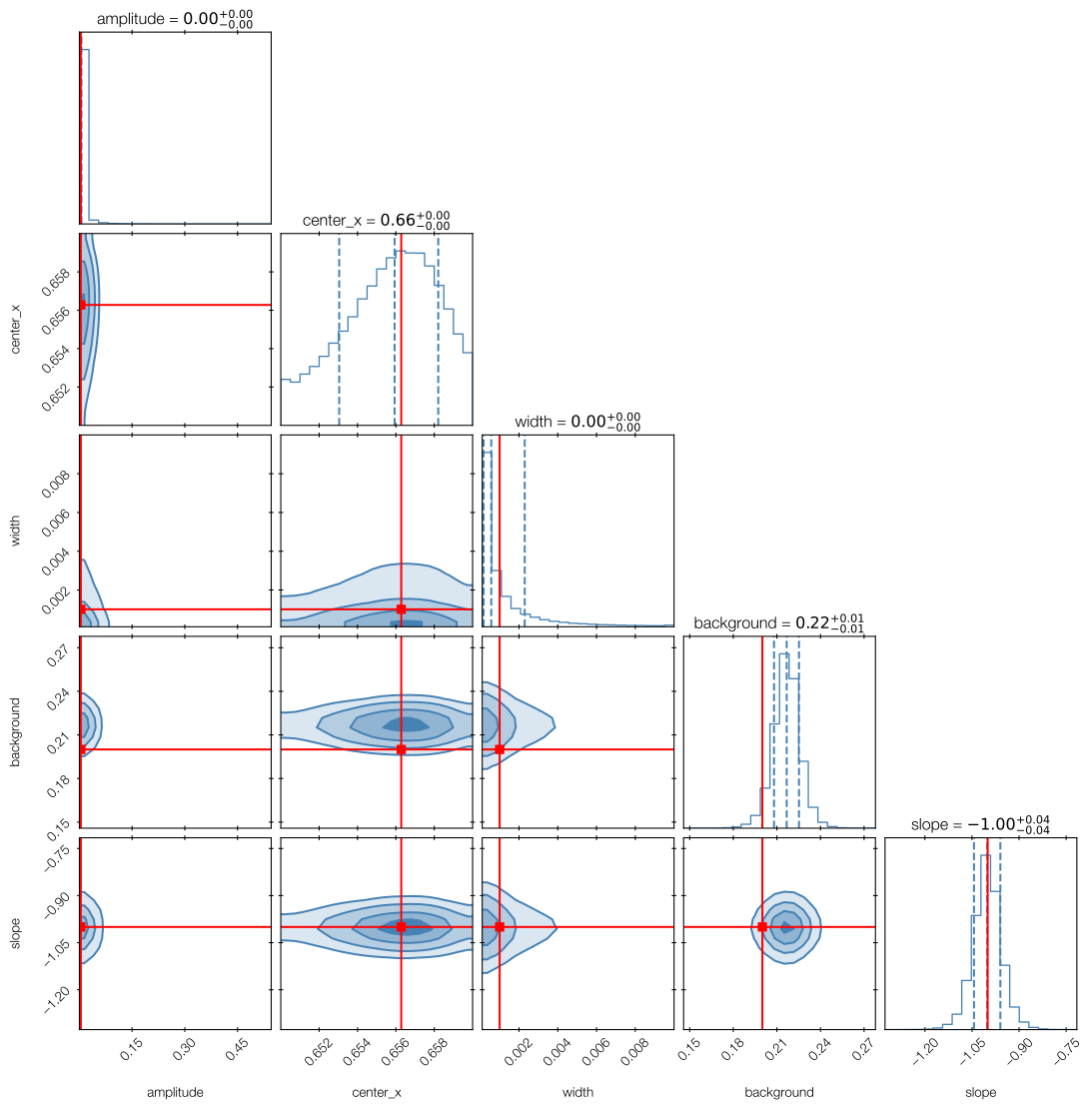
The neural posterior may loose a lot of information, may be biased, etc. We will check this below.

But let’s apply the neural model to our data and see what we get:

[21]:

from ultranest.simbase.minisbi.npe import sample_posterior

posterior_samples_u, posterior_samples_theta = sample_posterior(
    model=model,
    observed_data=obs_spectrum,
    prior_transform=prior_transform,
    n_params=N_PARAMS,
    n_posterior_samples=100000,
)


Predicted posterior (Kumaraswamy-Logistic product, unit-cube space):
  Param 0: loc=0.9722  scale=0.2069  a=1.1736  b=0.2353
  Param 1: loc=0.2995  scale=0.0911  a=1.4043  b=4.2954
  Param 2: loc=0.2332  scale=0.0886  a=1.8011  b=5.7020
  Param 3: loc=0.2467  scale=0.0056  a=0.0880  b=0.4349
  Param 4: loc=0.3481  scale=0.0134  a=0.4506  b=0.2955

[22]:

print("Posterior summary:")
for i, name in enumerate(parameter_names):
    samp = posterior_samples_theta[:, i]
    print(f"  {name:12s}: mean={samp.mean():.3f}  std={samp.std():.3f}"
          f"  true={theta_true[i]:.3f}")

Posterior summary:
  amplitude   : mean=0.005  std=0.016  true=0.004
  center_x    : mean=0.656  std=0.002  true=0.656
  width       : mean=0.001  std=0.002  true=0.001
  background  : mean=0.217  std=0.009  true=0.200
  slope       : mean=-1.002  std=0.046  true=-1.000

[23]:

corner.corner(
    posterior_samples_theta,
    labels=parameter_names,
    truths=theta_true,
    truth_color="red",
    show_titles=True,
    quantiles=[0.16, 0.5, 0.84],
    color="steelblue",
    plot_datapoints=False,
    fill_contours=True,
    smooth=1.0,
);

_images/example-simulation-based-inference_48_0.svg

Getting the NPE distribution parameters

The above is a Kumaraswamy-Logistic chained distribution defined on the unit hypercube. It can be summarized with a few distribution parameters for each model parameters.

[24]:

from ultranest.simbase.minisbi.nested import get_distribution_parameters, KLPTransform

[25]:

distribution_parameters = get_distribution_parameters(model, obs_spectrum)

[26]:

distribution_parameters

[26]:

{'loc': [0.972230076789856,
  0.29954269528388977,
  0.2332037091255188,
  0.24667471647262573,
  0.3480818271636963],
 'scale': [0.20693717896938324,
  0.09106920659542084,
  0.08857166767120361,
  0.005565132014453411,
  0.013386978767812252],
 'a': [1.1736023426055908,
  1.404343605041504,
  1.8011276721954346,
  0.08795655518770218,
  0.45056411623954773],
 'b': [0.23531001806259155,
  4.295437812805176,
  5.701991558074951,
  0.43487370014190674,
  0.29545164108276367]}

It might be useful to store for reuse:

[27]:

import json
with open(folder + '/distribution.json', 'w') as f:
    json.dump(distribution_parameters, f)

Checking the SBI model: rank histogram

First, we check that the model gives reliable posteriors, with a rank histogram.

We generate from the prior, and sample posterior samples. Ideally, the rank of the prior samples and the rank of the posterior samples are on a line (see Simulation-based calibration paper).

[28]:

from ultranest.simbase.minisbi.plot import rank_histogram

[29]:

ranks, fig, axes = rank_histogram(
    model=model,
    generate_noiseless_batch=generate_noiseless_batch,
    inject_noise=inject_noise,
    prior_transform=prior_transform,
    n_params=N_PARAMS,
    folder=folder,
    n_test=5000,
    seed=98765,
    param_names=parameter_names,
    n_bins=20,
)
fig;

Rank histogram:   0%|                                                                                                                   | 0/5000 [00:00<?, ?sim/s]/home/user/Downloads/UltraNest/ultranest/simbase/minisbi/logistic.py:39: RuntimeWarning: overflow encountered in exp
  return 1.0 / (1.0 + np.exp(-np.clip(x, -500.0, 500.0)))
Rank histogram: 100%|██████████████████████████████████████████████████████████████████████████████████████████████████████| 5000/5000 [00:00<00:00, 7402.33sim/s]

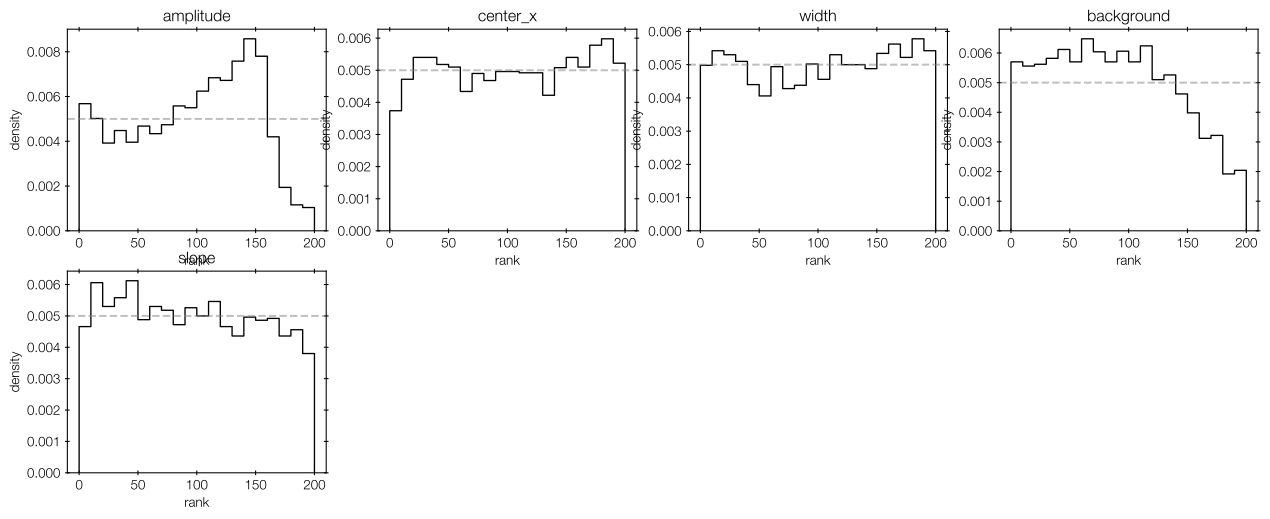
_images/example-simulation-based-inference_58_1.svg

These histograms should be flat.

If they a U-shaped, the posterior is over-confident. If they are inverse U-shaped, the posterior is under-confident.

You might be able to improve this by choosing a larger neural network.

[30]:

print("  Per-parameter rank statistics:")
for i, name in enumerate(parameter_names):
    print(f"    {name:12s}: mean={ranks[:, i].mean():.1f}  "
          f"std={ranks[:, i].std():.1f}  expected_mean=100.0")

  Per-parameter rank statistics:
    amplitude   : mean=95.9  std=51.1  expected_mean=100.0
    center_x    : mean=102.2  std=58.0  expected_mean=100.0
    width       : mean=101.7  std=59.0  expected_mean=100.0
    background  : mean=87.1  std=52.2  expected_mean=100.0
    slope       : mean=95.3  std=56.9  expected_mean=100.0

Checking the SBI model: coverage test

Next, we check whether the x% credible intervals contain the true value in x% of cases:

[31]:

from ultranest.simbase.minisbi.plot import parameter_coverage_test

[32]:

coverage, fig, axes = parameter_coverage_test(
    model=model,
    generate_noiseless_batch=generate_noiseless_batch,
    inject_noise=inject_noise,
    prior_transform=prior_transform,
    n_params=N_PARAMS,
    folder=folder,
    n_test=500,
    credible_levels=np.linspace(0.05, 0.99, 20).tolist(),
    seed=11223,
    param_names=parameter_names,
)
fig;

Coverage test:   0%|                                                                                                                     | 0/500 [00:00<?, ?sim/s]/home/user/Downloads/UltraNest/ultranest/simbase/minisbi/logistic.py:39: RuntimeWarning: overflow encountered in exp
  return 1.0 / (1.0 + np.exp(-np.clip(x, -500.0, 500.0)))
Coverage test: 100%|█████████████████████████████████████████████████████████████████████████████████████████████████████████| 500/500 [00:00<00:00, 6472.57sim/s]

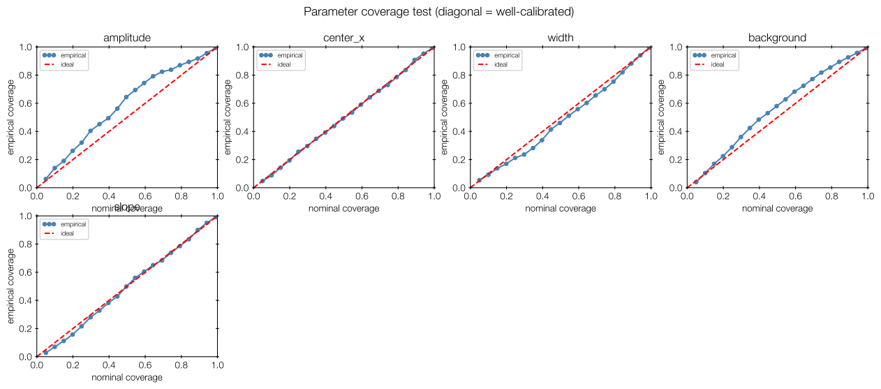
_images/example-simulation-based-inference_64_1.svg

These should follow the diagonal (red dashed).

Most of them look good. The amplitude parameter is slightly off, but not too wild.

If not, the posterior for that parameter is not well-calibrated (too narrow or too wide error bars). You might be able to improve this by choosing a larger neural network.

[33]:

print("  Empirical coverage at nominal 90% level:")
levels = np.linspace(0.05, 0.99, 20)
idx_90 = np.argmin(np.abs(levels - 0.90))
for i, name in enumerate(parameter_names):
    print(f"    {name:12s}: {coverage[idx_90, i]:.3f}  (nominal=0.900)")

  Empirical coverage at nominal 90% level:
    amplitude   : 0.918  (nominal=0.900)
    center_x    : 0.908  (nominal=0.900)
    width       : 0.882  (nominal=0.900)
    background  : 0.926  (nominal=0.900)
    slope       : 0.900  (nominal=0.900)

ultranest-sbi: SBI-accelerated nested sampling

Setting up the accelerated inference

Here we run nested sampling using the NPE posterior as a reparameterisation.

This allows nested sampling to start at a shrunk-down prior. To ensure identical inference as if we had started with the full prior, we need to correct the likelihood function by a penalty.

The nested sampler samples t ~ Uniform(0,1)^d.
The prior transform maps: t -> u -> theta
The log-likelihood includes a correction: loglike(theta) - log q(u | x_obs)

The correction ensures that the evidence integral and posterior samples are correct with respect to the original flat prior over u (and thus the physical prior over theta).

[34]:

# a helper object defining the distribution, its transform and log-posterior
klp_transform = KLPTransform(**distribution_parameters)

[35]:

class _State:
    last_t = None
state = _State()

# warp the prior by the NPE distribution
def warped_prior_transform(t):
    # keep the last state for likelihood
    state.last_t = t.copy()
    # [0,1]^d -> [0,1]^d with the SBI posterior warp
    u     = klp_transform.transform(t).astype(float)
    # [0,1]^d -> physical parameters
    theta = prior_transform(u)
    return theta

# correct the likelihood for the warp
def corrected_log_likelihood(theta):
    mp   = generate_mean_and_noise(theta=theta, idx=0, seed=0)
    # compute our model likelihood
    logL = loglikelihood(mp, obs_spectrum)
    # compute neural posterior density
    log_jac = klp_transform.log_jacobian(state.last_t)
    return logL + log_jac

Setting up the accelerated sampler

Build our accelerated ultranest-sbi sampler:

[36]:

sampler = ultranest.ReactiveNestedSampler(
    parameter_names,
    corrected_log_likelihood,
    warped_prior_transform,
    log_dir=folder,
    resume='overwrite',
)

Torch modified the logging to show all messages, let’s suppress that

[37]:

import logging

logger = logging.getLogger('ultranest')
logger.setLevel(logging.ERROR)
#logging.basicConfig(level=logging.INFO, stream=sys.stderr)

Run the accelerated ultranest-sbi sampler

[38]:

results = sampler.run(frac_remain=0.5, max_num_improvement_loops=0)

Z=873.6(47.43%) | Like=885.83..887.89 [885.8306..885.8338]*| it/evals=5160/16277 eff=32.4998% N=400

Posterior distribution:

Looking at the posterior distribution of the ultranest-sbi sampler, it is much narrower than the SBI one:

[39]:

corner.corner(
    results['samples'],
    labels=parameter_names,
    color="darkorange",
    plot_datapoints=False,
    fill_contours=False,
    smooth=1.0,
    contour_kwargs={"linestyles": "dashed"},
);

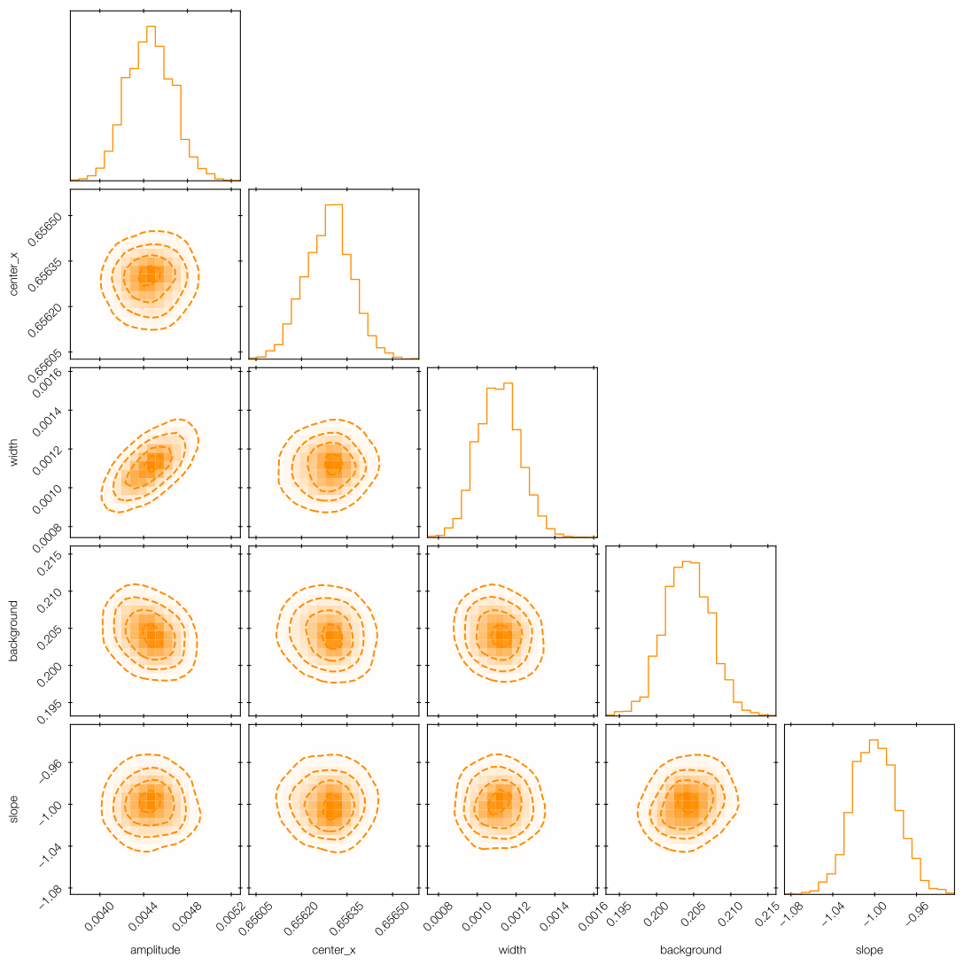
_images/example-simulation-based-inference_81_0.svg

Combined posterior distribution

Comparing them on the same plot, the SBI posterior is extremely wide, while ultranest manages to zoom in and get the full information.

[40]:

figure = corner.corner(
    posterior_samples_theta,
    labels=parameter_names,
    truths=theta_true,
    truth_color="red",
    show_titles=True,
    quantiles=[0.16, 0.5, 0.84],
    color="steelblue",
    plot_datapoints=False,
    fill_contours=True,
    smooth=1.0,
)
# overplot nested sampling posterior on the same figure
corner.corner(
    results['samples'],
    labels=parameter_names,
    fig=figure,
    color="darkorange",
    plot_datapoints=False,
    fill_contours=False,
    smooth=1.0,
    contour_kwargs={"linestyles": "dashed"},
);

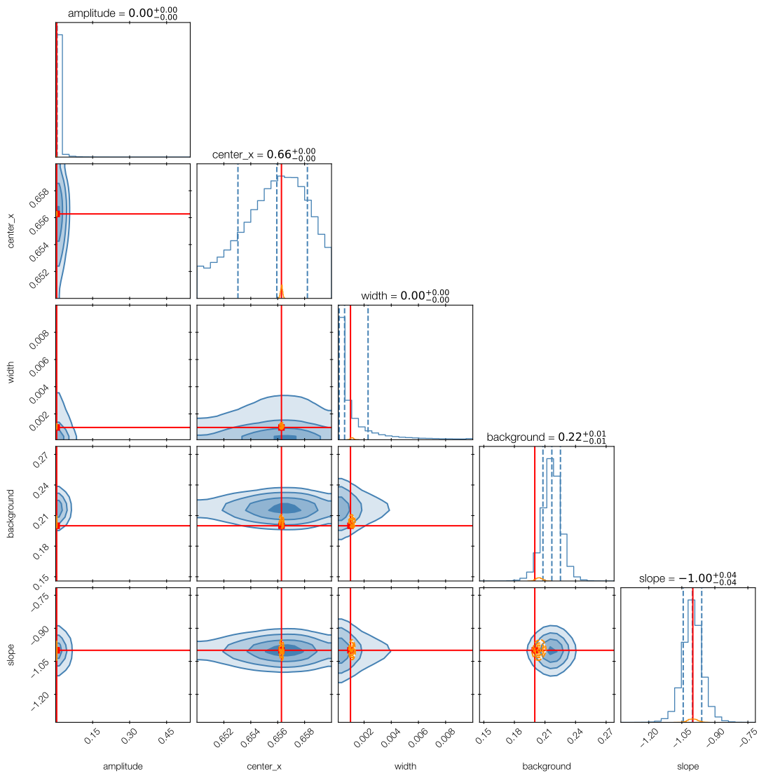
_images/example-simulation-based-inference_84_0.svg

Notice that the ultranest-sbi posterior (orange) is much narrower than the SBI posterior (blue), because SBI lost a lot of information. Nevertheless, the blue distribution provides a useful starting point for nested sampling.

Takeaways

In addition to the usual model and its likelihood, we defined a data simulator that can generate data.
We have learned to train a simulation-based inference (SBI) neural posterior estimator (NPE) model for obtaining a fast posterior distribution.
We checked that SBI posterior is amortized to behave well across the entire prior.
We used the SBI posterior on our data to get a starting point for a posterior distribution. This distribution has lost some information.
We used ultranest on top of the SBI posterior to get the posterior samples from the true posterior.
This ultranest-sbi approach effectively “skips” many initial nested sampling iterations, zooming into a data-driven guess for the posterior location. Because the SBI posterior is virtually always too wide, nested sampling is then fast to integrate to the actual posterior bulk.

Limitations: The posterior distribution used by the neural network is factorized and not optimal for challenging distributions. With a different, more sophisticated sbi package, better neural posteriors could be learned, but that would mean more complexity as well.

When using this in publications (such as legend entries), please refer to it as ultranest-sbi, to distinguish it from ultranest.

https://arxiv.org/abs/1804.06788, “Validating Bayesian Inference Algorithms with Simulation-Based Calibration”, Talts e al., 2018
https://doi.org/10.1073/pnas.1912789117 “The frontier of simulation-based inference”, Cranmer, Brehmer, Louppe, 2020