Visualisations
Advanced users will want to make their own visualisations and further analyses.
Loading the model
To start, lets pick one possible posterior sample:
posterior_sample = solver.posterior[0]
This will be the parameter values for each parameter:
for paramname, value in zip(solver.paramnames, posterior_sample):
        print(paramname, ":", value)
Next, we load the corresponding model:
# for sherpa:
for p, v in zip(solver.parameters, posterior_sample):
        p.val = v

# for xspec:
from bxa.xspec import set_parameters
set_parameters(transformations=solver.transformations, values=posterior_sample)
Getting the data for plotting
Now, you should use xspec or sherpa’s capabilities to make a plot, and extract the data.
For xspec, here are the references:
- https://heasarc.gsfc.nasa.gov/docs/xanadu/xspec/python/html/quick.html#plotting
see in particular the last example on that page!
https://heasarc.gsfc.nasa.gov/docs/xanadu/xspec/python/html/plotmanager.html#plotmanager-label
https://heasarc.gsfc.nasa.gov/docs/xanadu/xspec/python/html/extended.html#plotting
For sherpa, you probably want to use the get_model_plot (see also get_data_plot, get_source_plot, get_source_component_plot) to obtain the data to plot:
m = get_fit_plot()
y_model = m.modelplot.y
x_model = m.modelplot.x
x_data = m.dataplot.x
y_data = m.dataplot.y
yerr_data = m.dataplot.yerr
It may also be helpful to rebin the data prior to plotting.
Modifying the model
At this stage you could also extract information from a modified model.
For example, you could set the absorption to zero to plot the unabsorbed case, or remove nuisance components to reveal the key component of interest.
Getting the entire posterior
In the sections above, we have worked with one posterior sample, and obtained one model prediction.
For the Bayesian analysis, we have a posterior probability distribution of the parameters, so we also want a posterior distribution of our model plot.
The pattern to follow is:
prediction = []

for posterior_sample in solver.posterior:

        # load model (see above)
        ...

        # get plot data (see above)
        ...

        # save plot data from this realisation:
        prediction.append( ... )
Here, solver.posterior contains the equally weighted posterior samples (typically a few thousand). You can also limit yourself to a few hundred with solver.posterior[:400].
Plotting the prediction band
Finally, we want to plot the predictions.
This could be done inside the same script. Alternatively, you can write out the data to a text file and write a separate, dedicated plotting script that reads the data. This will allow you to quickly make changes to plots.
A helpful visualisation function to make credible interval bands is PredictionBand.
Putting it all together, here is one example for xspec:
from xspec import Plot
from bxa.xspec.solver import set_parameters, XSilence

band = None
Plot.background = True

with XSilence():
        Plot.device = '/null'
        # plot models
        for row in solver.posterior[:400]:
                set_parameters(values=row, transformations=solver.transformations)
                Plot('counts')
                if band is None:
                        band = PredictionBand(Plot.x())
                band.add(Plot.model())

band.shade(alpha=0.5)
band.shade(q=0.495, alpha=0.1)
band.line()

plt.scatter(Plot.x(), Plot.y(), label='data')
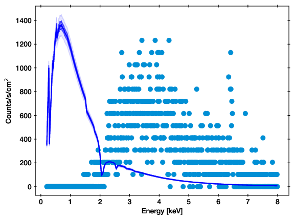
Example of the convolved model spectrum prediction band.
For an example of extracting plot data for sherpa, see the xagnfitter script (towards the bottom).
Fluxes and luminosities
Similar to extracting plots, you can also compute a flux or luminosity for each posterior sample, to obtain the entire posterior distribution.
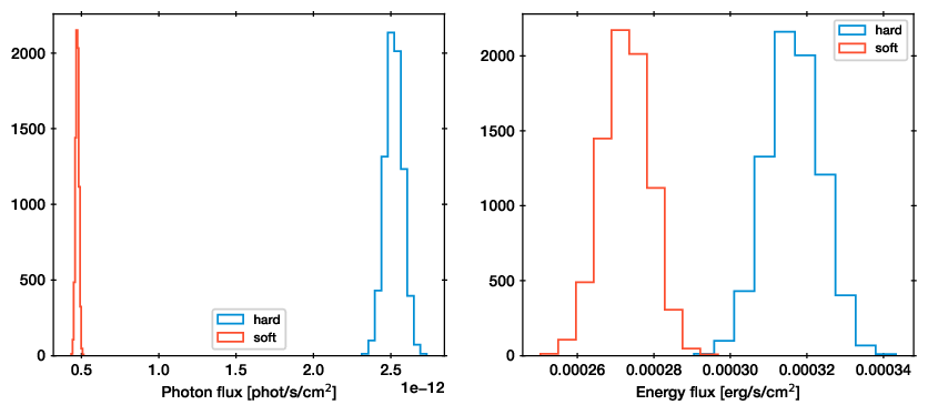
Posterior distribution of the soft and hard band fluxes. Photon fluxes are shown in the left panel, energy fluxes in the right panel. Histograms were obtained by taking each posterior sample, loading the model, then computing the flux.
Summary
On this page you learned the ingredients to load up model realisations, extract data and plot the results. Now you can make your visualisation the way you want it.
Visualisation contributions to BXA are welcome.