Sherpa with BXA

Begin by loading bxa in a session with sherpa loaded:

import bxa.sherpa as bxa

Defining priors

Define your background model and source model as usual in sherpa. Then define the priors over the free parameters, for example:

# three parameters we want to vary
param1 = xsapec.myapec.norm
param2 = xspowerlaw.mypowerlaw.norm
param3 = xspowerlaw.mypowerlaw.PhoIndex

# list of parameters
parameters = [param1, param2, param3]
# list of prior transforms
priors = [
   bxa.create_uniform_prior_for(param1),
   bxa.create_loguniform_prior_for(param2),
   bxa.create_gaussian_prior_for(param3, 1.95, 0.15),
   # and more priors
]

# make a single function:
priorfunction = bxa.create_prior_function(priors)

Make sure you set the parameter minimum and maximum values to appropriate (a priori reasonable) values. The limits are used to define the uniform and loguniform priors.

You can freeze the parameters you do not want to investigate, but BXA only modifies the parameters specified. As a hint, you can find all thawed parameters of a model with:

parameters = [for p in get_model().pars if not p.frozen and p.link is None]

You can also define your own prior functions, which transform unit variables unto the values needed for each parameter. See the UltraNest documentation on priors for more details about this concept. The script examples/sherpa/example_automatic_background_model.py gives an example of such a custom prior function (limited_19_24).

API information:

Prior Predictive Checks

To check that your priors and model is okay and working, create a flipbook of prior samples.

1. Pick a random sample from the prior:

   for parameter, prior_function in zip(parameters, priors):
            parameter.val = prior_function(numpy.random.uniform())
   

2. make a plot (plot_model, plot_source, etc.)

Repeat this 20 times and look at the plots.

Do the shapes and number of counts expected look like a reasonable representation of your prior expectation?

Running the analysis

You need to specify a prefix, called outputfiles_basename where the files are stored.

# see the pymultinest documentation for all options
solver = bxa.BXASolver(prior=priorfunction, parameters=parameters,
             outputfiles_basename = "myoutputs/")
results = solver.run(resume=True)

API information:

Parameter posterior plots

Credible intervals of the model parameters, and histograms (1d and 2d) of the marginal parameter distributions are plotted in ‘myoutputs/plots/corner.pdf’ for you.

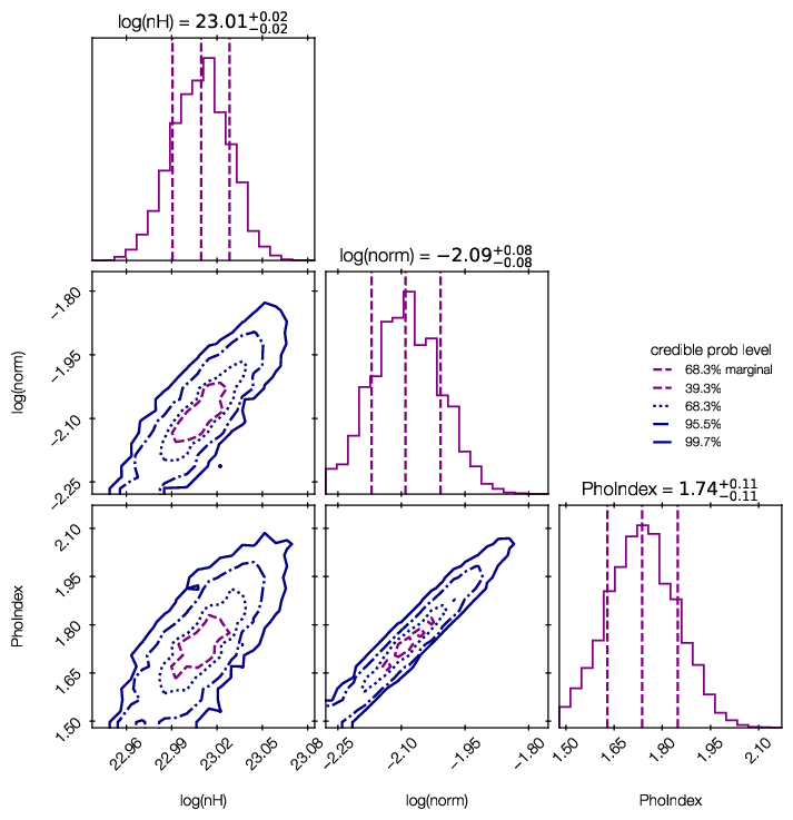
You can also plot them yourself using corner, triangle and getdist, by passing results[‘samples’] to them.

For more information on the corner library used here, see https://corner.readthedocs.io/en/latest/.

Error propagation

results[‘samples’] provides access to the posterior samples (similar to a Markov Chain). Use these to propagate errors:

• For every row in the chain, compute the quantity of interest

• Then, make a histogram of the results, or compute mean and standard deviations.

This preserves the structure of the uncertainty (multiple modes, degeneracies, etc.)

BXA also allows you to compute the fluxes corresponding to the parameter estimation, giving the correct probability distribution on the flux. With distance information (fixed value or distribution), you can later infer the correct luminosity distribution.

dist = solver.get_distribution_with_fluxes(lo=2, hi=10)
numpy.savetxt(out + prefix + "dist.txt", dist)

API information:

This does nothing more than:

r = []
for row in results['samples']:
        # set the parameter values to the current sample
        for p, v in zip(parameters, row):
                p.val = v
        r.append(list(row) + [calc_photon_flux(lo=elo, hi=ehi),
                calc_energy_flux(lo=elo, hi=ehi)])

Such loops can be useful for computing obscuration-corrected, rest-frame luminosities, (modifying the nH parameter and the energy ranges before computing the fluxes).

Model comparison

examples/xspec/model_compare.py shows an example of model selection. Keep in mind what model prior you would like to use.

• Case 1: Multiple models, want to find one best one to use from there on:

  • follow examples/model_compare.py, and pick the model with the highest evidence

• Case 2: Simpler and more complex models, want to find out which complexity is justified:

  • follow examples/model_compare.py, and keep the models above a certain threshold

• Case 3: Multiple models which could be correct, only interested in a parameter

  • Marginalize over the models: Use the posterior samples from each model, and weigh them by the relative probability of the models (weight = exp(lnZ))

Example output:

jbuchner@ds42 $ python model_compare.py absorbed/ line/ simplest/

Model comparison
****************

model simplest : log10(Z) = -1632.7  XXX ruled out
model absorbed : log10(Z) =    -7.5  XXX ruled out
model line     : log10(Z) =     0.0    <-- GOOD

The last, most likely model was used as normalization.
Uniform model priors are assumed, with a cut of log10(30) to rule out models.

jbuchner@ds42 $

Here, the probability of the second-best model, “absorbed”, is \(10^7.5\) times less likely than the model “line”. As this exceeds our threshold (by a lot!) we can claim the detection of an iron line!

Monte Carlo simulated spectra are recommended to derive a Bayes factor threshold for a preferred false selection rate. You can find an example in the Appendix of Buchner+14 and in the ultranest tutorial.

Experiment design

We want to to evaluate whether a planned experiment can detect features or constrain parameters, i.e. determine the discriminatory power of future configurations/surveys/missions.

For this, simulate a few spectra using the appropriate response.

• Case 1: Can the experiment constrain the parameters?

  • Analyse and check what fraction of the posterior samples lie inside/outside the region of interest.

• Case 2: Can the experiment distinguish between two models?

  • Model selection as above.

• Case 3: Which sources (redshift range, luminosity, etc) can be distinguished?

  • Compute a grid of spectra. Do model selection at each point in the grid.

Model discovery

Is the model the right one? Is there more in the data? These questions can not be answered in a statistical way, but what we can do is

1. generate ideas on what models could fit better

2. test those models for significance with model selection

For the first point, Quantile-Quantile plots provide a unbinned, less noisy alternative to residual plots.

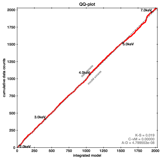
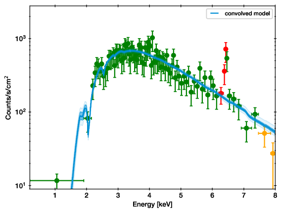
QQ plot example (left), with the corresponding spectrum for comparison (right).

In these plots, for each energy the number of counts observed with lower energy are plotted on one axis, while the predicted are on the other axis. If model and data agree perfectly, this would be a straight line. Deviances are indications of possible mis-fits.

This example is almost a perfect fit! You can see a offset growing at 6-7 keV, which remains at higher energies. This indicates that the data has more counts than the model there.

As the growth is in a S-shape, it is probably a Gaussian (see its cumulative density function).

Refer to the appendix of the accompaning paper for more examples.

The qq function in the qq module allows you to create such plots easily, by exporting the cumulative functions into a file.

Refer to the accompaning paper, which gives an introduction and detailed discussion on the methodology.