Example

SysCorr comes with a simple demonstration example in the example/ folder. We will go through the code.

Data

First, gen.py generates example data for analysis:

$ python gen.py

For instance, it creates the sysline/ dataset, which contains 40 datapoints:

$ ls sysline/chain
chain00  chain04  chain08  chain12  chain16  chain20  chain24  chain28  chain32  chain36
chain01  chain05  chain09  chain13  chain17  chain21  chain25  chain29  chain33  chain37
chain02  chain06  chain10  chain14  chain18  chain22  chain26  chain30  chain34  chain38
chain03  chain07  chain11  chain15  chain19  chain23  chain27  chain31  chain35  chain39

You can look at each data point, which is made up of a chain of values to represent the uncertainty (like a markov chain):

$ gnuplot
> plot [0:1] [-1:1] "sysline/chain01"

When you prepare your own data, make sure they are scaled so that they are in the units where you expect a relationship. I.e. if you are looking for a power law, take the logarithm of the values. If your x/y values lie outside the -20:20 range, you have to adapt the transform functions in the code (or scale the data).

Run

Launch the example application now:

$ RESUME=1 python analyse.py out/sysline_ sysline/chain??

This will take some time, so lets find out what the analysis.py file does. You will write a similar file for your application:

output_basename = sys.argv[1]
files = sys.argv[2:]
resume = os.environ.get('RESUME', '0') == '1'

1. The output will be written to ‘out/sysline_’ (first argument)
2. Files are the data files (second argument and onwards).
3. If you set RESUME=1, then the analysis will continue. Otherwise, it will start from scratch.

Models

Next, the models are defined:

example_models = dict(
	# y is drawn independently of x, from a gaussian. 2 free parameters (stdev, mean)
	independent_normal = PolyModel(1, rv_type = scipy.stats.norm),

	# y is drawn independently of x, from a uniform dist. 2 free parameters (width, low)
	independent_uniform = PolyModel(1, rv_type = scipy.stats.uniform),

	# y is drawn as a function of x, with gaussian systematic scatter 
	# y ~ N(b*x + a, s)      3 free parameters (s, a, b)
	line = PolyModel(2),

	# y is drawn as a function of x, with gaussian systematic scatter 
	# y ~ N(c*x**2 + b*x + a, s)      4 free parameters (s, a, b, c)
	square = PolyModel(3),
	
	# two gaussians before and after 0. 4 parameters (means and stdevs)
	tribinned = BinnedModel(bins = [(-0.5, 0.3), (0.3, 0.8), (0.8, 1.5)], rv_type = scipy.stats.norm)
)

If you want to compare a linear correlation to a non-correlation, you would have ‘independent_uniform’ and ‘line’.

The next code chunk just allows you to specify models from the command line without editing code:

modelnames = os.environ.get('MODELS', '').split()
if len(modelnames) == 0:
	modelnames = example_models.keys()

models = []
for m in modelnames:
	print 'using model:', m
	model = example_models[m]
	models.append((m, model))

Calculation

All that is left is to load the data and send it off!

print 'loading data...'
chains = [(f, numpy.loadtxt(f)) for f in files]
print 'loading data done.'

syscorr.calc_models(models=models, 
	chains=chains, 
	output_basename=output_basename, 
	resume=resume)

Output

As an example, the text output can look like this:

(...)
Total Samples:                              8011
Nested Sampling ln(Z):                -38.456223
 ln(ev)=  -38.109756655272683      +/-  0.13633196813580595
 Total Likelihood Evaluations:         8011
 Sampling finished. Exiting MultiNest
  analysing data from out/sysline_independent_normal.txt
Analysing multinest output...
  analysing data from out/sysline_independent_normal.txt
posterior plot written to "out/sysline_independent_normalpost_model_data.pdf"

calculation results: ========================================

          model name | log Z
 independent_uniform : -21.8
  independent_normal : -16.6
           tribinned : -11.3
              square : -7.9
                line : -6.7 <- BEST MODEL

Parameters for model "line":
            syserror: 0.18+/-0.04
                   a: 1.8+/-0.2
                   b: 0.17+/-0.08

This gives you the best model (line), and the parameters of that line. (Input was y=2*x + 0.1 with error 0.1)

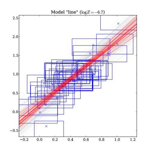
The model with several permitted parameters overplotted over the data. For each model prediction, red is the median line, while grey shows the 10%/90% quantiles. The data points are shown in blue using the x/y median and the permitted x/y extrema for the rectangles.

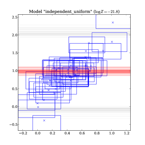
Same as above, but for the model with independent uniform distribution for y, i.e. y is uncorrelated of x. This model is ruled out by the model selection (see text output above).